INTRODUCTION

Analyzing texts is an essential part of natural language processing and plays a crucial role in determining various tasks such as sentiment analyses, classification, recommendation systems, content summarization, machine translation, question-answering-based systems and much more. In this Blog, we shall delve into 2 major text representation techniques - Count Vectorizer and TF-IDF along with a word embedding technique - Word2Vec

DATASET

In this Blog, we shall use the Twitter Dataset for a better understanding. We shall be using the 'text' column of the dataset to understand all the concepts discussed in the blog.

COUNT VECTORIZER v/s TF-IDF

Count Vectorizer is one of the simplest easy-to-understand techniques that converts a collection of text documents (sentences) into a matrix of word/token counts. Each row in the matrix represents a text document that varies across the columns which are all the unique words contained in the entire corpus!

Have a quick look at the image below :

In the first document, we see that the words "bird" 5 times and the words "about" and "the" occur once and twice respectively. This technique helps us determine the frequency of words in the text document. Similarly, all the text documents are converted to numerical values which are of potential use to various machine learning/NLP models.

Code Snippet :

#Load the count vectorizer from sklearn library, and various other libraries such as pandas
import pandas as pd
from sklearn.feature_extraction.text import CountVectorizer

#Read the dataset from the csv file 
tweet=pd.read_csv("twcs.csv")

#Load the text column from the twitter dataset
text=tweet['text']

#Create an instance of the CountVectorizer class from sklearn
#We remove the stop words using all the predefined stop words in english as they are of less significance
#We convert all the alphabets to lower case as all the words irrespective of their case should be treated equally.
#We are specifying maximum number of features to be 15 to consider the top 15 most imp words
#Below we have set the configuration of the Count_vectorizer to the terms defined above
cv=CountVectorizer(stop_words='english', lowercase=True, max_features=15)
fit_transform= cv.fit_transform(text)

#Count vectorizer does 3 things: Tokenization, Counting and Vectorization
#Tokenization: It breaks down words in a sentence into tokens/unique words
#Counting: It counts the frequency of each word in the text/sentence
#Vectorization: It represents the text data in a matrix form where
#rows represents the occurance of words and columns represents the words in the documents/sentences

features = cv.get_feature_names_out()
features

#We are counting the word frequency along the columns and converting the matrix to a 1d array
word_counts = fit_transform.sum(axis=0).A1

#Create a dataframe with the frequency and words
df= pd.DataFrame({'Word': features, 'Count': word_counts})
result1 = result_df.head(15)
result_df = df.sort_values(by='Count', ascending=False)

#display the top 15 words
print(result1)

Output :

The code above gives us the frequency of the most occurring words in the entire text document of the Twitter dataset.

Pros :

1. Simplicity: It is a straightforward technique, easy to implement and understand.

2. Interpretability: Easy to interpret the results as they are a matrix representation of word frequencies.

Cons :

1. Word semantics: Ignores the meaning of words, which can limit its performance in tasks requiring semantic understanding.

2. High dimensionality: The resultant matrix can become extremely high dimensional due to its nature leading to computational challenges.

Term Frequency-Inverse Document Frequency better known as TF-IDF is an advanced text representation technique that considers the importance of words in the document relative to their frequency in the entire series of text. Words that are frequent but rare in the corpus receive higher scores which indicates their significance.

Code Snippet:

from sklearn.feature_extraction.text import TfidfVectorizer

tdidf=TfidfVectorizer(stop_words='english',lowercase=True,max_features=50)
fit_transform=tdidf.fit_transform(text)

features=tdidf.get_feature_names_out()
tfidfs=fit_transform.sum(axis=0).A1
result = pd.DataFrame({'Word': features, 'Score': tfidfs})

# Sort the DataFrame by TF-IDF score in descending order
result= result.sort_values(by='Score', ascending=False)

# Get the top 50 most frequent words
result2 = result.head(50)

print(result2)

Output :

The code above gives us the frequency score of the most significant words in the dataset.

I shall display the difference in word selection below:

Code snippet:

#As we can see here the resultant datafram containing both the pevious dataframes obtained from the Count Vectroizer and TD-IDF are compared
#We conclude that the results have slight variations when using TD-IDF since the model takes the term freq and how unique the word is across each document unlike countvectorizer which only looks at term frequencies across the all documents
#TD-IDF finds content specific words which are important in each document, hence depending on a particular task we can decide if TD-IDF or Count vextorizer is better

result1.reset_index(drop=True, inplace=True)
result2.reset_index(drop=True, inplace=True)

# Concatenate DataFrames along columns (axis=1)
final= pd.concat([result1, result2], axis=1)
final.head(10)

Output:

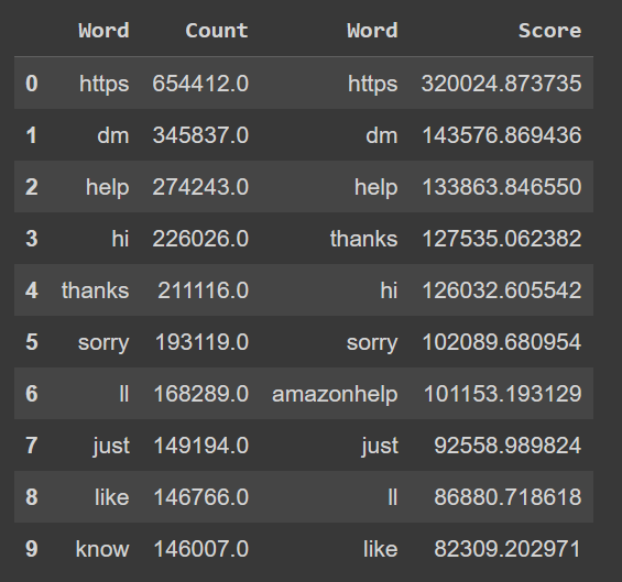
As we can see from the above outputs generated, both techniques work slightly differently.

Pros :

1. Semantic Understanding: Since this method considers both word frequency and document specificity, it provides a better representation of the document's content.

2. Dimensionality: It focuses more on the significant terms hence the TF-TDF has a reduced dimensionality.

Cons:

1. Complexity: Could be a more complex model to implement

2. Word Order: Not ideal to capture the word order which may limit its performance in tasks like sentiment analysis.

WORD2VEC: EMBEDDING MODEL

The essence of the word embedding model developed by Tomas Mikolov and his team at Google lies in learning the semantic meanings of words from their co-occurrence patterns.

This model uses a neural network to map words to high-dimensional vectors where words with similar meanings tend to be collected together.

Using the model's architecture, we can predict the target word based on the surrounding context words. For example: " The Dog ran and sat on a" Would predict the next word to be "couch".

Advantages of word2vec model:

1. Semantic relationship: This model understands the semantic meaning of words, for example, "queen - women + man" = King

2. Computation: It has a low dimensionality hence it requires fewer computational resources, making it more efficient.

from gensim.models import Word2Vec
word2vec_model = Word2Vec(sentences, vector_size=100, window=5, min_count=1, sg=0)
word2vec_model.save("word2vec.model")

word2vec_model = Word2Vec.load("word2vec.model")

#Search for similar words using the models that we trained to the ones that we got using count vectorizer (top 15)
similar_words = {}
for word in top_words:
    similar_words[word] = {
        "Word2Vec": word2vec_model.wv.most_similar(word),
        "FastText": fasttext_model.wv.most_similar(word),
        "Glove_model": glove_model.most_similar('word', topn=5)
    }

The above code Snippet gives us the words familiar to the words /sentences we feed in!

Conclusion

In the vast ocean of text data, our journey has taken us through the powerful techniques of Count vectorization, TF-IDF and Word2Vec models. Each of these with its unique strengths offers an array of possibilities for text analysis, natural language processing and machine learning.

You may find the full code used in this blog on my GitHub page.

I hope you enjoyed learning about these powerful NLP tools. Feel free to explore and adapt the code to your specific needs. Happy coding !!