What is ARIMA?

ARIMA, also known as an "Autoregressive Integrated Moving Average" model is a time series forecasting Machine learning technique that is widely used in industries such as finance(stock market prediction, exchange rates), marketing(customer demands, sales trends), economics(GDP, inflation) and many others.

Breaking down ARIMA

To understand the term ARIMA "Autoregressive Integrated Moving Average", we shall split it into 3 Parts. The "Autoregressive" part of the model utilizes the past values of the time series data to predict future values. The "Integrated" part takes care of the process called differencing, which is used if the dataset is not stationary. Again we shall talk about differencing in the later part of the blog. The "Moving Average" is part of the model which uses the previous forecast errors to predict future values.

What is SARIMAX?

SARIMAX, Stands for "Seasonal Autoregressive Integrated Moving Average with Exogenous Regressors" and is mainly used to predict values for a given seasonal dataset.

How to identify seasonal data?

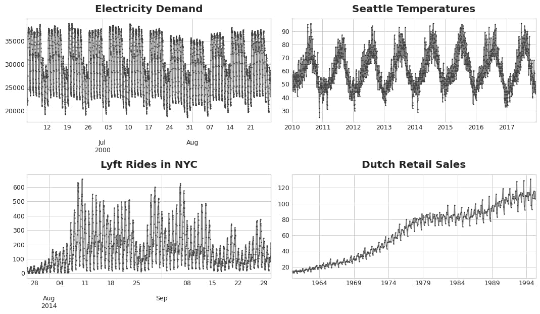
Seasonal data repeats over a specific period. All 4 images displayed below are examples of seasonal data.

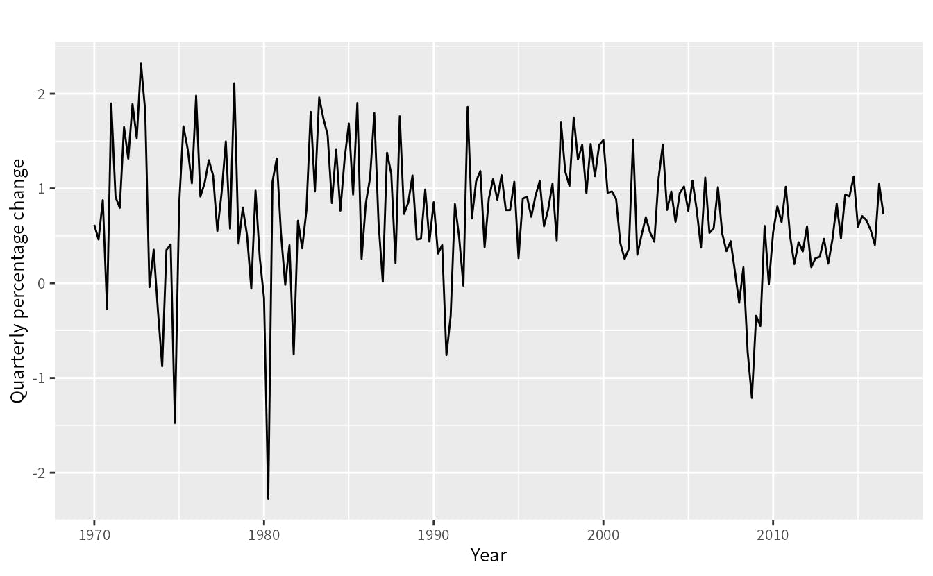
Whereas, the image below is an example of a nonseasonal dataset.

Code:

Now that you guys know when to use ARIMA(Seasonal) and SARIMAX(nonseasonal), let's code to find out how it works :

Note: The dataset and the code are available on my Github, profile.

Preprocess the dataset

Step 1: Install all the necessary libraries and dependencies

#Import all the necessary libraries 
!pip install pmdarima
import numpy as np #Used for numpy arrays
import pandas as pd #Used to utilize the pandas dataframe 
from statsmodels.tsa.stattools import adfuller #Helps us perform the Dickey fuller test
from pmdarima import auto_arima #This library helpds us decide the parameter (order) for our ARIMA/SARIMAX models
import statsmodels.api as sm # Import the SARIMAX Model
from pandas.tseries.offsets import DateOffset

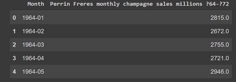
Step 2: Import the dataset and rename the columns if necessary:

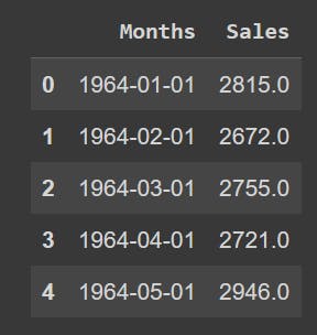
This dataset contains 2 columns: "Month" and "Perrin Freres monthly champagne sales millions ?64-?72".

dataframe=pd.read_csv('dataset.csv') # Read the dataset 
dataframe.head() #Display the first few values
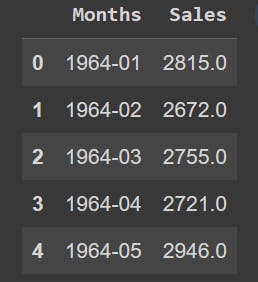
dataframe.columns=["Months","Sales"] #Rename the columns for better understanding
df = dataframef[dataframe['Sales'].notna()] #Remove the Null values from the column 'Sales' in the dataset
df.head() #Display the first few values

Step 3: Convert the dates column to datetime format using pandas.

df['Months']=pd.to_datetime(df['Months']) #Convert to datetime format
df.head() #Display few values of the dataset

Step 4: Convert the "Months" column as index values

df.set_index('Months', inplace=True)

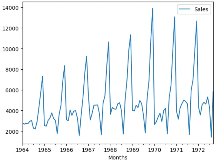
Step 5: Visualize the graph of the Preprocessed Dataset

df.plot() #Displays the seasonality for every year

Test To find out whether the dataset is stationary or not:

Step 1: We will assume a Null Hypothesis which states that the dataset is nonstationary and the Alternate Hypothesis states that the dataset is stationary.

#Ho: It is non stationary
#H1: It is stationary
#If the P value is lesser that 0.05, the Null hypothesis is rejected and vice versa
dftest = adfuller(df['Sales', autolag = 'AIC') #Perform the Dickey Fuller test 
print("1. ADF : ",dftest[0])
print("2. P-Value : ", dftest[1])
print("3. Num Of Lags : ", dftest[2])
print("4. Num Of Observations Used For ADF Regression:",dftest[3])
print("5. Critical Values :")
for key, val in dftest[4].items():
    print("\t",key, ": ", val)

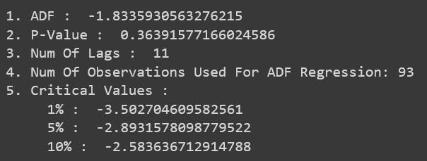
Step 2: Since the p-value is higher than 0.05 the Null Hypothesis is right and hence the dataset is not stationary. To make the dataset stationary we do "Differencing". Since our data is seasonal(every year), we do differencing by 12 months.

df["Seasonal_Shift"]=df["Sales"].shift(12) #Create a new column Seasonal Shift and fill it with values that are shifted by 12 months verticially.
df["Difference"]=df["Sales"]-df["Seasonal_Shift"] #Add a new column "Difference to display the difference between Sales(Original) and the Seasonal_Shift(Shifted) values 
new_df = df[df['Difference'].notna()] #Drop the na values 
new_df['Difference'].plot() #Plot the difference

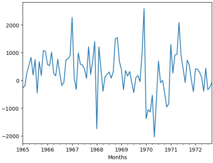
We can see that the above plot is stationary with no trends.

Step 3: Run Autorima on the Sales Values to get the best order for p,d,q Values to run our SARIMAX model

Values= auto_arima(new_df['Difference'], trace=True) #Find out the best  values for p,d and q through auto_arima
Values.summary()#Get a summary for it

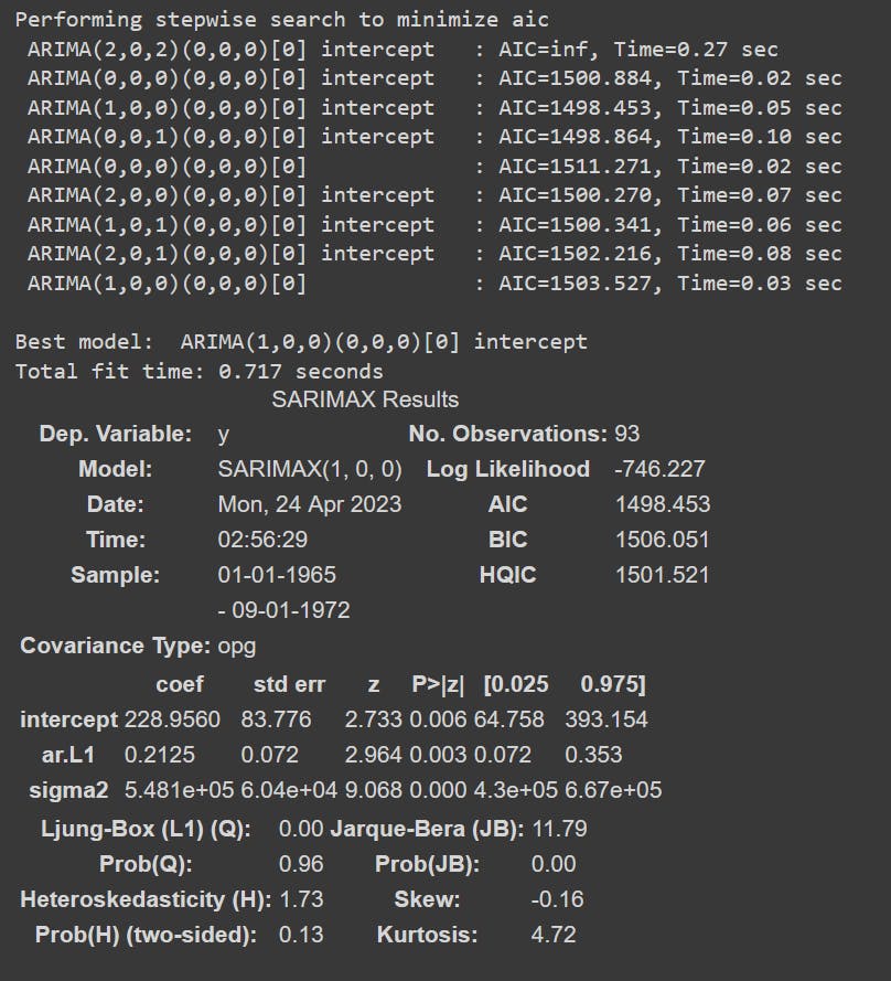
The best values provided by our Autoarima model for our p,d and q values are 1,0 and 0 respectively.

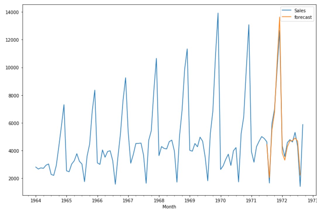
Step 4: Fit the SARIMAX model to our Sales Data with the order (1,0,0) and seasonal shift of 12.

model=sm.tsa.statespace.SARIMAX(new_df['Sales'],order=(1, 0, 0),seasonal_order=(1,0,0,12)) #Fit the model into SARIMAX witht he order 1,0,0
results=model.fit()
df['forecast']=results.predict(start=70,end=103,dynamic=True) #Predicted values
df[['Sales','forecast']].plot(figsize=(12,8))#Plot the Sales Value

Step 5: Predict the Future Values

date=[df.index[-1]+ DateOffset(months=x)for x in range(0,24)] 
dataframe=pd.DataFrame(index=date[1:],columns=df.columns)
future_df=pd.concat([new_df,dataframe])
future_df['forecast'] = results.predict(start = 104, end = 120, dynamic= True)  
future_df[['Sales', 'forecast']].plot(figsize=(12, 8))

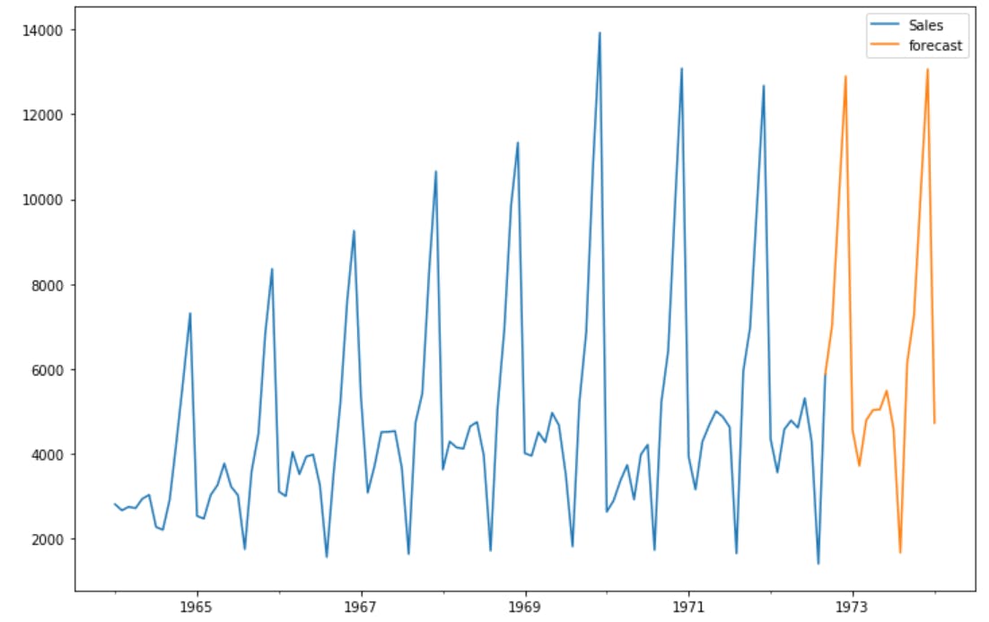
We finally have the predicted values for the SARIMAX model. Similarly, if the dataset is not seasonal, we can use the ARIMA model to forecast and predict future values.

While the concept of ARIMA may seem daunting at first, the availability of packages in R and Python has made it more accessible than ever before. By following the best practices for model selection, tuning and evaluation one can leverage ARIMA models to extract insights and drive business outcomes efficiently.